The standard error of estimate sounds like the kind of statistic that wears a lab coat, speaks only in Greek letters, and refuses to explain itself at dinner. Thankfully, it is much friendlier than it looks. If you can subtract, square numbers, add them up, divide, and take a square root, you can calculate it.
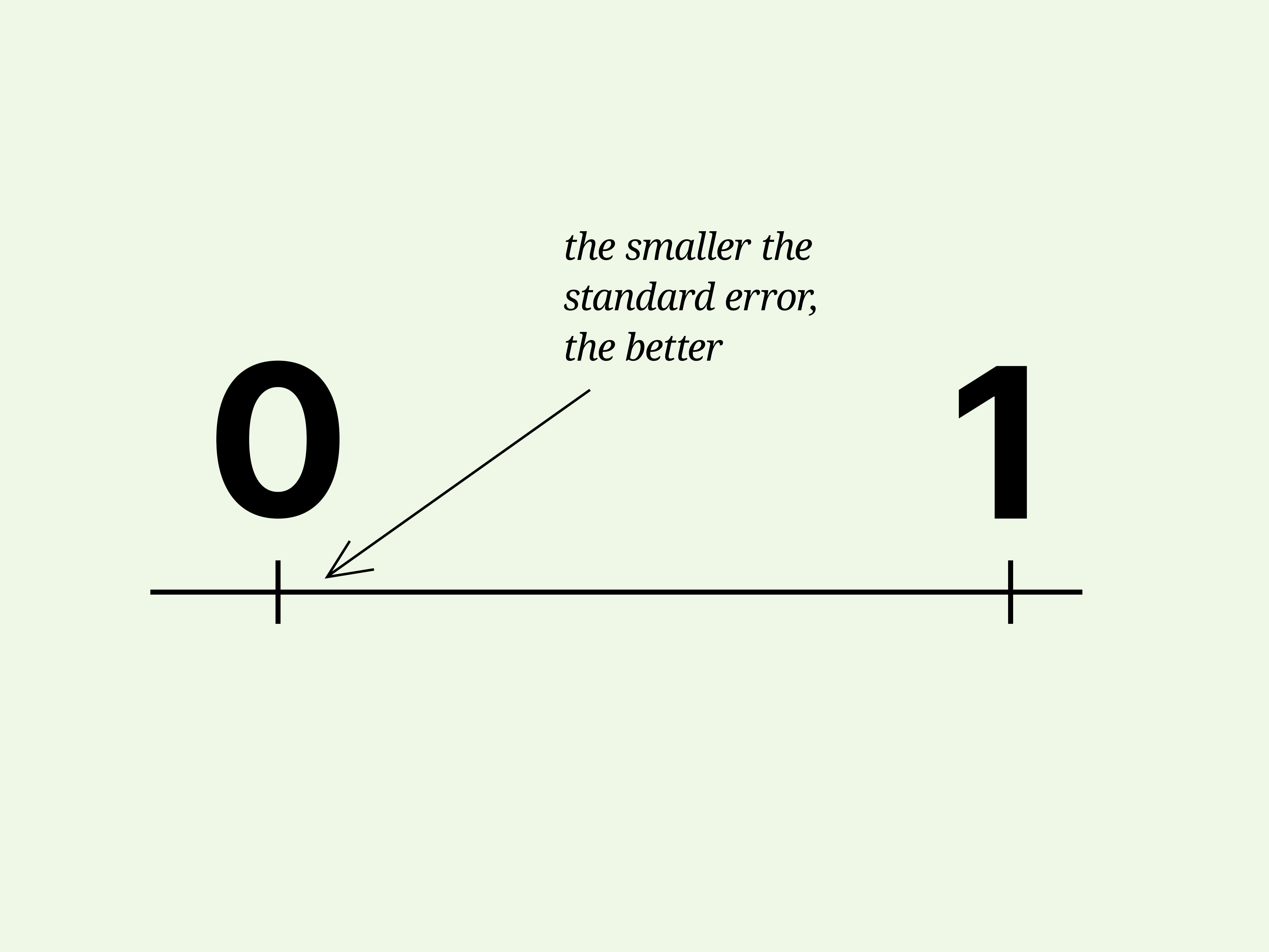
In plain English, the standard error of estimate tells you how far your actual data points typically fall from a regression line. It is commonly used in linear regression to measure the accuracy of predictions. When the number is small, your regression model is making predictions that sit close to the real values. When the number is large, your model is wandering around like it forgot where it parked.
This guide walks you through the meaning, formula, calculation steps, examples, interpretation, common mistakes, and practical experience behind the standard error of estimate. Whether you are working on a statistics assignment, business forecast, research project, or data analysis report, this article will help you calculate and explain the result clearly.
What Is the Standard Error of Estimate?
The standard error of estimate, often abbreviated as SEE, measures the typical size of the errors made by a regression model. In simple linear regression, the model creates a straight line that predicts a dependent variable, usually called y, from an independent variable, usually called x.
For every actual value of y, the regression line produces a predicted value, written as ŷ. The difference between the actual value and the predicted value is called a residual:
Residual = Actual value – Predicted value
The standard error of estimate summarizes those residuals into one useful number. Instead of staring at a long list of errors, you get a single value that says, “On average, the model’s predictions are off by about this much.”
Why the Standard Error of Estimate Matters
The standard error of estimate is important because prediction is the whole point of many regression models. A model may have a nice-looking equation, a tidy chart, and a confident spreadsheet, but if its predictions are often far away from reality, it is not very useful.
SEE helps answer practical questions such as:
- How accurate is this regression model?
- How far are the actual values from the predicted values?
- Can this model be trusted for forecasting?
- Is one regression model more precise than another?
- Are the prediction errors small enough for the problem I am solving?
For example, a standard error of estimate of 2 pounds in a weight prediction model may be excellent. But a standard error of estimate of 2 million dollars in a small-business revenue forecast may cause several people to suddenly need coffee.
The Standard Error of Estimate Formula
For simple linear regression, the standard error of estimate formula is:
SEE = √[Σ(y – ŷ)2 / (n – 2)]
Here is what each part means:
- y = actual observed value
- ŷ = predicted value from the regression equation
- y – ŷ = residual or prediction error
- Σ(y – ŷ)2 = sum of squared errors, also called SSE
- n = number of observations
- n – 2 = degrees of freedom for simple linear regression
The reason we divide by n – 2 instead of simply n is that a simple linear regression model estimates two parameters: the intercept and the slope. Those two estimated values use up two degrees of freedom.
Formula for Multiple Regression
If your model has more than one independent variable, the formula changes slightly:
SEE = √[SSE / (n – k – 1)]
In this version, k is the number of independent variables. The extra 1 accounts for the intercept. For example, if you use three predictors, the denominator is n – 3 – 1, or n – 4.
How to Calculate the Standard Error of Estimate Step by Step
Now let’s turn the formula into something easier to follow. The calculation is not hard, but the order matters. Think of it like baking: flour before frosting, residuals before square root.
Step 1: Create or Identify the Regression Equation
First, you need a regression equation. In simple linear regression, the equation usually looks like this:
ŷ = a + bx
Here, a is the intercept and b is the slope. The equation predicts y based on x.
For example:
ŷ = 51 + 6.4x
This means the predicted y value starts at 51 when x is zero, and increases by 6.4 for every one-unit increase in x.
Step 2: Calculate the Predicted Values
Next, plug each x value into the regression equation to get each predicted value, or ŷ.
Suppose we are predicting test scores from hours studied. Our regression equation is:
ŷ = 51 + 6.4x
If a student studied 3 hours, the predicted score would be:
ŷ = 51 + 6.4(3) = 70.2
Step 3: Find Each Residual
Now subtract the predicted value from the actual value:
Residual = y – ŷ
If the actual score was 71 and the predicted score was 70.2, the residual is:
71 – 70.2 = 0.8
A positive residual means the actual value was higher than predicted. A negative residual means the actual value was lower than predicted.
Step 4: Square Each Residual
Residuals can be positive or negative. If we simply added them, positive and negative errors could cancel each other out, which would make the model look better than it really is. Sneaky? Yes. Useful? No.
To solve that problem, square each residual:
Squared residual = (y – ŷ)2
Step 5: Add the Squared Residuals
Add all squared residuals together. This gives you the sum of squared errors, or SSE:
SSE = Σ(y – ŷ)2
SSE is the total unexplained error left after the regression model has made its predictions.
Step 6: Divide by the Degrees of Freedom
For simple linear regression, divide SSE by n – 2:
SSE / (n – 2)
This gives you the average squared error after adjusting for the two estimated regression parameters.
Step 7: Take the Square Root
Finally, take the square root of the result. This converts the answer back into the original units of y.
If y is measured in dollars, SEE is measured in dollars. If y is measured in points, SEE is measured in points. That makes interpretation much easier.
Standard Error of Estimate Example
Let’s calculate SEE using a small example. Suppose we have five students, and we want to predict test scores based on hours studied.
| Hours Studied (x) | Actual Score (y) | Predicted Score (ŷ) | Residual (y – ŷ) | Squared Residual |
|---|---|---|---|---|
| 1 | 58 | 57.4 | 0.6 | 0.36 |
| 2 | 63 | 63.8 | -0.8 | 0.64 |
| 3 | 71 | 70.2 | 0.8 | 0.64 |
| 4 | 75 | 76.6 | -1.6 | 2.56 |
| 5 | 84 | 83.0 | 1.0 | 1.00 |
Now add the squared residuals:
SSE = 0.36 + 0.64 + 0.64 + 2.56 + 1.00 = 5.20
There are five observations, so n = 5. Because this is simple linear regression, divide by n – 2:
5.20 / (5 – 2) = 5.20 / 3 = 1.7333
Now take the square root:
SEE = √1.7333 = 1.32
The standard error of estimate is approximately 1.32 test score points. That means the model’s predictions are typically off by about 1.32 points. For a small classroom example, that is a pretty tight fit. The model earns a gold star, or at least a very respectable sticker.
How to Interpret the Standard Error of Estimate
The standard error of estimate should always be interpreted in the units of the dependent variable. If your dependent variable is home price, SEE is in dollars. If your dependent variable is delivery time, SEE is in minutes. If your dependent variable is exam score, SEE is in points.
A lower SEE generally means the regression line fits the data better. A higher SEE means the actual values tend to fall farther away from the predicted values.
Example Interpretation
Suppose a regression model predicts monthly sales and has a standard error of estimate of $4,000. You could explain it like this:
“The model’s sales predictions typically differ from actual monthly sales by about $4,000.”
That statement is much easier to understand than saying, “The square root of the mean squared residual adjusted for degrees of freedom is 4,000.” Both are technically connected, but one sounds like a helpful analyst and the other sounds like a calculator trapped in a cave.
Standard Error of Estimate vs. R-Squared
The standard error of estimate and R-squared both evaluate regression models, but they answer different questions.
R-squared tells you the percentage of variation in y explained by the model. It is a relative measure. For example, an R-squared of 0.80 means the model explains 80% of the variation in the dependent variable.
Standard error of estimate tells you the typical prediction error in the original units of y. It is an absolute measure.
Both are useful. R-squared tells you how much variation the model explains. SEE tells you how far off the predictions are in real-world terms. If you are presenting results to non-statisticians, SEE is often easier to understand because it uses familiar units.
Standard Error of Estimate vs. Standard Error of the Mean
Do not confuse the standard error of estimate with the standard error of the mean. They sound similar, but they are used for different purposes.
The standard error of the mean measures how precisely a sample mean estimates a population mean. The standard error of estimate measures how accurately a regression model predicts values.
In short:
- Standard error of the mean: about estimating an average
- Standard error of estimate: about prediction errors in regression
Standard Error of Estimate vs. RMSE
The standard error of estimate is closely related to root mean square error, or RMSE. Both summarize prediction errors by using squared residuals and a square root.
The main difference is often the denominator. RMSE may divide by n, especially in machine learning contexts. The standard error of estimate in regression divides by the residual degrees of freedom, such as n – 2 in simple linear regression or n – k – 1 in multiple regression.
That degrees-of-freedom adjustment makes SEE especially appropriate when you are estimating a regression model from sample data.
Common Mistakes When Calculating SEE
Using Actual Values Instead of Residuals
SEE is based on the differences between actual and predicted values, not the actual values alone. Always calculate y – ŷ first.
Forgetting to Square the Residuals
If you do not square the residuals, positive and negative errors can cancel out. That can make a messy model look suspiciously perfect.
Dividing by n Instead of n – 2
For simple linear regression, divide by n – 2. For multiple regression, divide by n – k – 1. Using the wrong denominator changes the result.
Ignoring the Units
SEE is only meaningful when interpreted in the units of the dependent variable. A SEE of 5 may be tiny for income measured in dollars but huge for a satisfaction score measured from 1 to 10.
Comparing SEE Across Different Outcomes
Do not compare a SEE for house prices with a SEE for test scores. The units are completely different. Compare SEE values only when the dependent variable is the same or has been properly standardized.
When Is a Standard Error of Estimate “Good”?
There is no universal number that makes SEE good or bad. A good SEE depends on the context, the scale of y, the purpose of the model, and the cost of prediction errors.
For example, if a shipping model predicts delivery time with a SEE of 3 minutes, that might be excellent. If a medical dosage model has an error large enough to create unsafe recommendations, that is not acceptable. Context is the boss.
Ask these questions when judging SEE:
- Is the error small compared with the typical value of y?
- Would this level of error be acceptable in real decisions?
- Is this model better than a simpler model?
- Do the residual plots show random scatter?
- Are there outliers heavily influencing the result?
How to Reduce the Standard Error of Estimate
If your SEE is too high, your model may need improvement. Here are practical ways to reduce prediction error:
- Add relevant predictors: A missing variable may explain part of the variation.
- Remove irrelevant predictors: Extra noise can weaken model performance.
- Check for nonlinear patterns: A straight line may not fit curved data well.
- Investigate outliers: Extreme values can inflate residual error.
- Transform variables: Log or square-root transformations may improve fit for skewed data.
- Collect better data: No formula can rescue messy, biased, or incomplete data forever.
However, do not chase a tiny SEE at any cost. A model can overfit the data, meaning it performs beautifully on the current dataset but poorly on new data. That is like memorizing the answer key and then panicking when the teacher changes the questions.
Practical Experience: What Calculating SEE Teaches You
Working with the standard error of estimate in real projects teaches a lesson that formulas alone cannot: prediction error is not an embarrassment. It is information. Every residual tells you something about where your model is strong, where it struggles, and where the data may be more complicated than the equation suggests.
One of the most useful experiences is learning to inspect the residuals before celebrating the final SEE value. A model may have a reasonably low standard error of estimate, but the residuals may reveal a pattern. For example, the model may underpredict small values and overpredict large values. That pattern suggests the relationship may not be truly linear. In that case, the SEE is still useful, but it is not the whole story.
Another practical lesson is that SEE feels different depending on the audience. In a classroom, you may calculate it because the assignment asks for it. In business, the number becomes a decision-making tool. If a sales forecast has a SEE of $20,000, a manager immediately wants to know whether that level of error is acceptable. If monthly sales are usually $2 million, maybe the error is manageable. If monthly sales are usually $30,000, that same SEE is a five-alarm spreadsheet fire.
In data analysis work, SEE is also helpful because it encourages humility. A regression equation may look exact, especially when displayed with several decimal places, but the standard error reminds you that predictions come with uncertainty. That is a good thing. Responsible analysts do not pretend their models are crystal balls. They explain the likely size of the error so others can make smarter decisions.
A strong habit is to report SEE alongside R-squared. R-squared may impress people because percentages feel clean and confident, but SEE translates model performance into real units. Saying “the model explains 82% of the variation” is useful. Saying “the model is typically off by about 4.6 units” is often more practical. Together, the two statistics give a fuller picture.
Another experience worth noting is that smaller is not always automatically better. If you add many predictors, the model may fit the current sample more closely, but it may become harder to explain and less reliable on new data. In real-world modeling, simplicity has value. A slightly higher SEE may be acceptable if the model is easier to maintain, easier to communicate, and more stable.
Calculating SEE by hand at least once is also surprisingly useful. Software can produce the number instantly, but manual calculation shows what is happening behind the scenes. You see the actual values, predicted values, residuals, squared residuals, SSE, degrees of freedom, and square root all working together. After that, regression output no longer looks like a mysterious machine. It looks like organized arithmetic with a statistics badge.
The final practical takeaway is simple: use SEE as a reality check. When the number is small and residuals look random, your regression model may be doing a good job. When the number is large or residuals show patterns, the model is asking for more attention. Listen to it. Data may not speak in complete sentences, but residuals are definitely trying to tell you something.
Conclusion
The standard error of estimate is one of the clearest ways to measure prediction accuracy in regression. It tells you the typical distance between actual values and predicted values, using the same units as the dependent variable. To calculate it, find the residuals, square them, add them to get SSE, divide by the correct degrees of freedom, and take the square root.
For simple linear regression, use SEE = √[Σ(y – ŷ)2 / (n – 2)]. For multiple regression, use SEE = √[SSE / (n – k – 1)]. A smaller SEE generally means a better-fitting model, but context matters. The best analysts do not just calculate the number; they interpret it, compare it carefully, check residuals, and explain what it means in real-world language.
Once you understand SEE, regression becomes less intimidating. It is not just a line on a chart. It is a prediction tool with a built-in honesty meter.