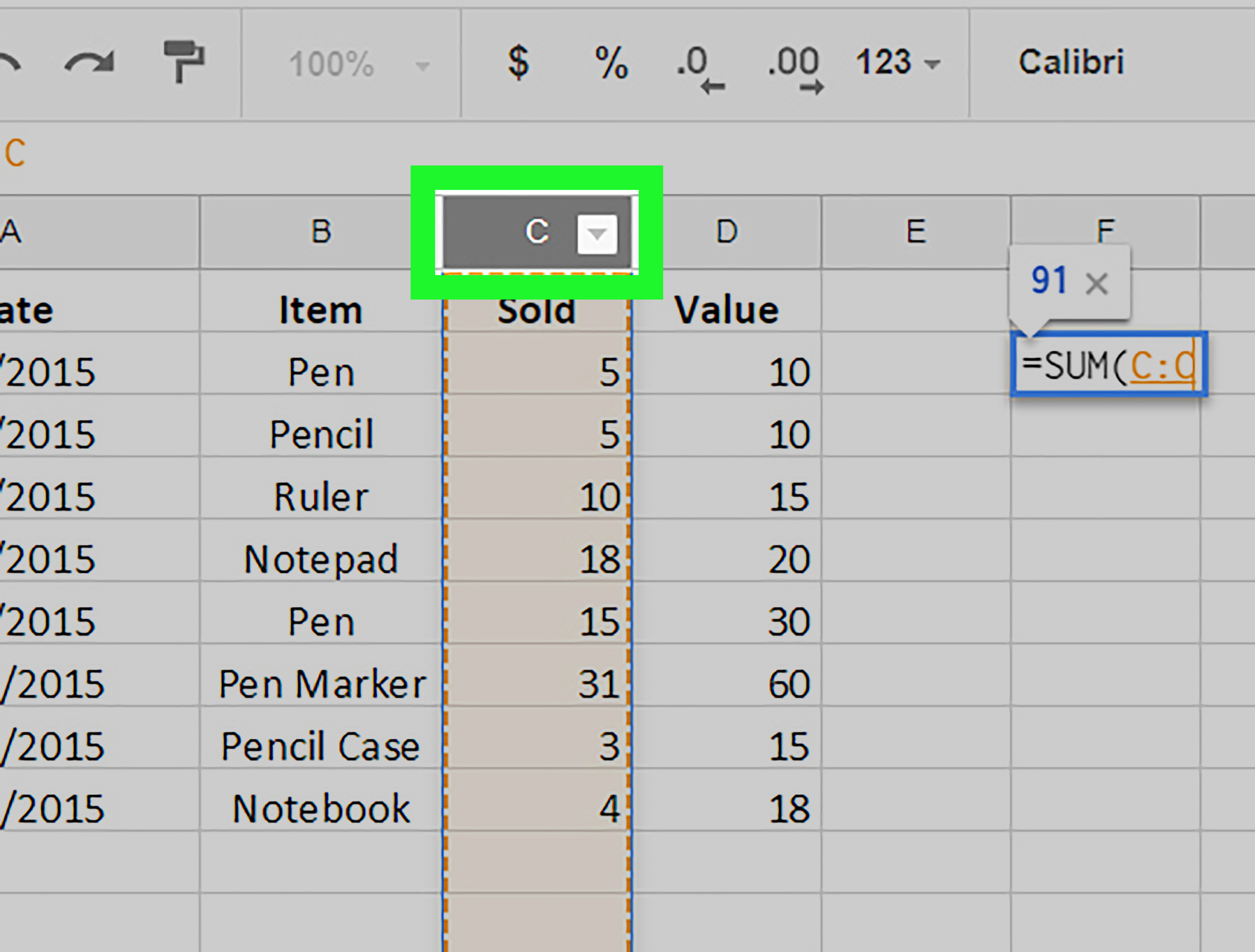
Apply a Formula to a Column in Google Sheets

Applying a formula to an entire column in Google Sheets sounds like one of those tiny spreadsheet chores that should take three seconds. Then you drag the fill handle, overshoot by 4,000 rows, accidentally copy the formula into your notes column, and suddenly your peaceful spreadsheet has become a small office crime scene.

The good news: Google Sheets gives you several clean ways to apply a formula to a whole column on a PC or Mac. You can drag the fill handle, double-click it, use keyboard shortcuts, copy and paste, or let ARRAYFORMULA do the heavy lifting automatically. The best method depends on whether you want the formula to apply only to existing rows or continue working when new rows are added later.

This guide explains each method in plain English, with examples, troubleshooting tips, and practical advice for choosing the right approach. Whether you are calculating totals, combining names, adding tax, tracking commissions, or cleaning messy imported data, these steps will help you make Google Sheets behave like a helpful assistant instead of a stubborn calculator with commitment issues.

Why Apply a Formula to an Entire Column in Google Sheets?

Most spreadsheets are built around repeated calculations. If row 2 calculates a sales total, row 3 probably needs the same logic. So does row 4. And row 5. And, depending on your job, row 5,000 may also be sitting there waiting patiently for a formula.

Applying a formula to an entire column saves time, improves consistency, and reduces manual errors. Instead of typing the same formula again and again, you create it once and let Google Sheets repeat the pattern. This is especially useful for tasks like:

Multiplying quantity by price
Calculating profit margins
Combining first and last names
Changing text formatting
Adding dates, tax, fees, or discounts
Checking whether a row meets a condition
Cleaning imported data from forms or apps

For example, if column A contains product prices and column B contains quantities, you might use this formula in cell C2:

That formula calculates the total for row 2. To apply the same logic down the column, you need Google Sheets to adjust the row numbers automatically: A3*B3, A4*B4, A5*B5, and so on. This is where fill tools, shortcuts, and array formulas become extremely useful.

Method 1: Use the Fill Handle to Drag the Formula Down

The fill handle is the small square or dot in the bottom-right corner of a selected cell. It may look humble, but it is basically the tiny blue steering wheel of spreadsheet productivity.

How to use the fill handle on PC or Mac

Open your spreadsheet in Google Sheets.
Click the first cell where you want the formula result to appear.
Type your formula. For example: =A2*B2
Press Enter.
Click the formula cell again.
Move your cursor to the bottom-right corner of the cell until the fill handle appears.
Click and drag the fill handle down the column.
Release your mouse when you reach the last row you want to fill.

Google Sheets copies the formula into the selected cells and adjusts relative references automatically. So if C2 contains =A2*B2, dragging it down to C3 changes the formula to =A3*B3. This is exactly what you want for row-by-row calculations.

When this method works best

Dragging the fill handle is ideal for smaller datasets or one-time tasks. If your sheet has 20, 100, or even a few hundred rows, it is quick and easy. The downside is that dragging becomes annoying when your data runs for thousands of rows. Nobody opens Google Sheets dreaming of a mouse-dragging marathon.

Method 2: Double-Click the Fill Handle

If your formula column sits next to a column that already contains data, you can often double-click the fill handle instead of dragging it manually. This is one of the fastest ways to copy a formula down an entire column of existing rows.

How to double-click the fill handle

Enter your formula in the first row of the output column.
Click the cell containing the formula.
Move your cursor to the bottom-right corner of the cell.
Double-click the fill handle.

Google Sheets will fill the formula down based on the neighboring data range. For example, if column A has data from A2 through A250, and your formula is in C2, double-clicking the fill handle may copy the formula down to C250.

Why double-clicking sometimes stops early

The double-click method depends on nearby data. If the adjacent column has blank cells, Sheets may stop filling earlier than expected. Imagine Google Sheets walking down the rows, seeing an empty cell, and saying, “Well, I guess we are done here.”

If double-clicking does not fill the entire range, check for blank rows or use one of the other methods below.

Method 3: Use Keyboard Shortcuts to Fill Down

Keyboard shortcuts are perfect when you want speed without playing target practice with the fill handle. On Windows, ChromeOS, and most PC keyboards, the fill-down shortcut is Ctrl + D. On Mac, it is usually Command + D.

How to fill down with a shortcut

Type your formula in the first cell of the column.
Select that formula cell and the cells below it where you want the formula copied.
Press Ctrl + D on PC or Command + D on Mac.

Google Sheets fills the selected range using the formula from the top cell. This method is especially useful when you already know the exact range you want to fill.

Example

Suppose C2 contains:

Select C2:C100, then press Ctrl + D or Command + D. Sheets copies the formula down through C100 and updates the row references automatically.

Method 4: Copy and Paste the Formula Into the Entire Column

Copy and paste is not fancy, but it works. Sometimes the reliable old method is the right method, like wearing sneakers instead of trying to roller-skate through a grocery store.

How to copy and paste a formula down a column

Enter the formula in the first cell.
Copy the cell with Ctrl + C on PC or Command + C on Mac.
Select the destination range in the same column.
Paste with Ctrl + V or Command + V.

Google Sheets will adjust relative references as it pastes the formula into each row. If you paste =A2*B2 from C2 into C3, the formula becomes =A3*B3.

When copy and paste is useful

This method is helpful when you want to fill formulas into a specific range, non-adjacent cells, or a filtered section. However, be careful when working with filtered data. Pasting into filtered rows can behave differently depending on what is selected, so always check a few results afterward.

Method 5: Use ARRAYFORMULA to Apply a Formula Automatically

If you want the formula to apply to current and future rows automatically, ARRAYFORMULA is usually the best choice. Instead of copying a formula into hundreds of cells, you place one formula at the top of the output column, and it spills results down the column.

Think of ARRAYFORMULA as the spreadsheet version of “set it and stop babysitting it.”

Basic ARRAYFORMULA example

Instead of entering this in C2 and dragging down:

You can enter this in C2:

This tells Google Sheets to multiply each value in column A by the matching value in column B, starting from row 2. The results appear down column C automatically.

Add a blank-row check

The basic version may show zeros or unwanted results for empty rows. To keep the output clean, wrap the formula with IF:

This formula says: if column A is blank, show a blank result; otherwise, multiply column A by column B. Much tidier. Your spreadsheet will look less like it spilled numbers everywhere.

ARRAYFORMULA for combining text

If column A has first names and column B has last names, use:

This combines first and last names for every row. For example, “Maya” in A2 and “Johnson” in B2 becomes “Maya Johnson” in C2.

ARRAYFORMULA with IF logic

Suppose column B contains scores, and you want column C to show “Pass” for scores of 70 or higher and “Review” for lower scores:

This is excellent for grading sheets, sales qualification lists, project status trackers, and any spreadsheet where rules need to apply consistently across many rows.

Which Method Should You Choose?

The best method depends on your goal. If you only need to fill existing rows once, the fill handle or keyboard shortcut is fast. If you expect new rows to be added later, especially from Google Forms, Zapier, imports, or manual entries, ARRAYFORMULA is usually better.

Use the fill handle when:

Your dataset is small or medium-sized.
You only need the formula for existing rows.
You are comfortable dragging or double-clicking.
You want each cell to contain its own separate formula.

Use keyboard shortcuts when:

You already selected the destination range.
You prefer keyboard speed over mouse dragging.
You are filling a clearly defined section of rows.

Use ARRAYFORMULA when:

You want one formula to control the whole column.
New rows will be added over time.
You want to avoid copying formulas again later.
You are building a cleaner, more automated spreadsheet.

Understanding Relative and Absolute References

Before filling formulas down a column, it helps to understand how references behave. In Google Sheets, a reference like A2 is relative. When you copy it down one row, it becomes A3. That is helpful when each row needs its own calculation.

An absolute reference uses dollar signs, like this:

This locks the reference so it does not change when copied. You can lock only the column, only the row, or both:

A2 changes by row and column.
$A$2 always points to A2.
$A2 locks column A but allows the row to change.
A$2 locks row 2 but allows the column to change.

Example with a fixed tax rate

Suppose prices are in column A, and the tax rate is stored in E1. In B2, you might write:

When you fill this down, A2 becomes A3, A4, and so on, but $E$1 stays fixed. This is exactly what you want when every row uses the same tax rate.

Common Problems and How to Fix Them

The formula does not fill all the way down

If double-clicking the fill handle stops early, check the neighboring columns for blank rows. Google Sheets uses nearby data to guess where the fill should end. Blank cells can interrupt that guess.

ARRAYFORMULA shows results in too many rows

If an array formula fills thousands of blank rows with zeros or repeated output, add a blank check:

This keeps empty rows clean until data appears.

You see a “Result was not expanded” error

This usually means cells below the array formula are not empty. An array formula needs space to spill its results. Clear the cells below the formula, then try again.

The formula gives the same result in every row

Check whether you used absolute references by accident. If every row points to $A$2 and $B$2, every row will calculate the same thing. Use relative references like A2 and B2 when each row should calculate its own data.

The formula is slow

Full-column references like A2:A are convenient, but very large sheets with many complex array formulas can slow down. If performance becomes a problem, limit the range to a realistic size, such as A2:A1000, or simplify the formula.

Practical Examples for Everyday Google Sheets Work

Calculate total sales

If column A contains prices and column B contains quantities, enter this in C2:

Add a 10% fee

If column A contains original prices, use:

Create email addresses from names

If column A has first names and column B has last names, use:

Mark rows as complete

If column D contains completion dates, use:

Best Practices for Applying Formulas to Columns

Use headers clearly. A formula column should have a label that explains the result, such as “Total,” “Status,” “Full Name,” or “Commission.” Future you will appreciate this. Future coworkers will appreciate it even more.

Keep formulas in predictable locations. If you use ARRAYFORMULA, place it in the first result cell under the header, usually row 2. Avoid mixing manual entries into the same output column because they can block the array formula from expanding.

Test formulas on a few rows first. Before applying a formula to an entire column, confirm that it works correctly in one row. A tiny mistake copied into 10,000 rows is still tiny, technically, but it becomes emotionally large.

Use blank checks for cleaner sheets. Formulas like IF(A2:A="", "", calculation) prevent unnecessary output in empty rows. This makes your sheet easier to read and reduces confusion.

Document complicated formulas. If your formula includes multiple conditions, lookups, or text functions, consider adding a note in the header cell or a separate documentation tab. Spreadsheets age better when humans can still understand them six months later.

My Experience: What Actually Works Best in Real Google Sheets Projects

After working with many Google Sheets setups, the biggest lesson is simple: the “best” way to apply a formula to an entire column depends less on the formula and more on how the sheet will be used. A quick personal budget sheet, a sales tracker, and a form-connected operations dashboard all need different levels of automation.

For small, personal spreadsheets, I usually start with the fill handle. It is fast, visual, and hard to overthink. If I have a list of 40 expenses and want to multiply each amount by a tax rate, dragging the formula down is perfectly fine. There is no need to bring in a giant formula cannon when a simple click-and-drag will do the job.

For business sheets, I prefer ARRAYFORMULA whenever new rows are expected. This is especially true for sheets connected to Google Forms or automation tools. New form submissions often appear as new rows, and regular copied formulas do not always follow them automatically. Without an array formula, someone eventually has to notice that the last 83 rows are missing calculations. That person is usually tired, under-caffeinated, and not emotionally prepared for spreadsheet detective work.

One of the most useful habits is building formulas with blank-row protection from the beginning. For example, instead of using =ARRAYFORMULA(A2:A*B2:B), I prefer =ARRAYFORMULA(IF(A2:A="", "", A2:A*B2:B)). That small condition keeps the column clean and avoids a long trail of zeros. It also makes the sheet look more professional, which matters when clients, managers, or teammates open it.

Another experience-based tip: do not use full-column array formulas everywhere just because you can. They are powerful, but too many complex formulas across entire columns can slow down a large workbook. If you know the sheet will never exceed 2,000 rows, it is reasonable to use a limited range like A2:A2000. This keeps calculations lighter while still giving you plenty of room.

I have also learned to be careful with absolute references. Many formula problems come from locking the wrong part of a reference. If a tax rate, exchange rate, or commission percentage lives in one fixed cell, lock it with dollar signs. But if each row should use its own value, do not lock the row number. A formula copied perfectly with the wrong reference is still wrong; it is just wrong very efficiently.

For shared team sheets, I like using one array formula per calculated column and protecting that formula cell if needed. This prevents well-meaning teammates from pasting over formulas. Spreadsheet chaos often comes from good intentions wearing muddy shoes.

Finally, always check the first result, a middle result, and the last result after applying a formula to an entire column. This quick three-point check catches most mistakes. Look for blank rows, strange zeros, repeated values, and formulas that stop too early. A minute of checking can save an afternoon of wondering why the report says your company sold negative 17 chairs.

Conclusion

Applying a formula to an entire column in Google Sheets on PC or Mac is easy once you know your options. For quick one-time work, drag the fill handle, double-click it, use fill-down shortcuts, or copy and paste the formula into the range you need. For automated sheets that grow over time, ARRAYFORMULA is usually the smarter choice because it lets one formula handle an entire column dynamically.

The key is choosing the method that matches your workflow. Small sheet? Fill handle. Defined range? Keyboard shortcut. Constantly growing data? Array formula. Shared business tracker? Use clean formulas, blank checks, and protected cells. Your spreadsheet should work for you, not demand daily tribute like a tiny grid-shaped emperor.

Once you understand relative references, absolute references, and the difference between copied formulas and array formulas, Google Sheets becomes much easier to control. You will spend less time dragging, fixing, and muttering at cells, and more time actually using your data.