Excel is wonderful at storing long product names, customer notes, tracking codes, addresses, messy imports, and descriptions that look like they were typed by a keyboard wearing mittens. But sometimes you do not need the entire text string. You only need the first 10 characters, the last few digits, the part before a dash, or a cleaner version that fits nicely into a report without stretching the worksheet into the next ZIP code.
That is where learning how to truncate text in Excel becomes useful. In simple terms, truncating text means shortening it by keeping only the part you need. You can do this with formulas, modern text functions, or built-in Excel tools that require no formulas at all. The best method depends on whether your text has a predictable character count, a clear delimiter, or a pattern Excel can recognize.
This guide explains three practical ways to truncate text in Excel, with examples you can copy, adapt, and use right away. We will cover fixed-length truncation, delimiter-based truncation, and no-formula options such as Flash Fill, Text to Columns, and Power Query. Your spreadsheet will still be a spreadsheet, but at least the text will stop behaving like an overexcited paragraph.
What Does “Truncate Text in Excel” Actually Mean?
Before jumping into formulas, it helps to separate two common ideas. First, you may want to visually cut off text so it does not spill across nearby cells. That is a formatting issue. You can adjust column width, wrap text, shrink text, or hide overflow by placing content in the next cell. This changes how text appears, not the actual value inside the cell.
Second, you may want to truly shorten the text value. For example, turning PROD-45892-WINTER-BLUE into PROD-45892 changes the data itself. This is real truncation. It is useful for cleaning imported records, creating shorter labels, extracting IDs, preparing reports, and making large datasets easier to search, filter, and analyze.
The methods below focus mainly on real truncation, but we will also mention display-related tips where they make sense. The goal is not to make Excel look pretty for five minutes. The goal is to make your data behave better for the long haul.
Way 1: Truncate Text by Character Count with LEFT, RIGHT, and MID
The most direct way to truncate text in Excel is to tell Excel exactly how many characters to keep. This works best when your data follows a consistent structure. If every product code begins with a five-character prefix, or every tracking number ends with a four-digit batch code, fixed-length formulas are fast, clean, and dependable.
Use LEFT to Keep Characters from the Beginning
The LEFT function returns characters from the start of a text string. Its basic structure is:
Suppose cell A2 contains this value:
To keep only the first eight characters, use:
The result is:
This is handy for invoice prefixes, category codes, department abbreviations, shortened names, or any situation where the useful part begins on the left side of the cell.
Use RIGHT to Keep Characters from the End
The RIGHT function does the opposite. It keeps characters from the end of the text string:
If A2 contains:
and you want only the final four digits, use:
The result is:
This method is especially useful for extracting ZIP code endings, batch numbers, invoice endings, last four digits of an ID, or file extensions when the length is predictable.
Use MID to Extract Text from the Middle
The MID function lets you start at a specific character position and keep a specific number of characters:
If A2 contains:
and you want the three-letter color code beginning at character 5, use:
The result is:
MID is useful when your text has a stable structure, such as a SKU format, internal code, date stamp, or location identifier. It is less ideal when the length of the text before the target value changes from row to row.
Remove Characters from the End with LEFT and LEN
Sometimes you do not want to keep a fixed number of characters. Instead, you want to remove a fixed number of characters from the end. That is where LEN joins the party. The LEN function counts the number of characters in a cell.
If A2 contains:
and you want to remove the last four characters, use:
The result is:
This is a favorite formula for removing suffixes, trailing codes, extra characters, or unwanted endings. It is flexible because it adapts to the length of each cell rather than assuming every entry has the same total number of characters.
Way 2: Truncate Text Before or After a Delimiter
Fixed character counts are great when your data is neat. Unfortunately, real-world Excel files often arrive looking like someone tossed a salad made of names, dashes, commas, spaces, and mystery symbols. In that case, truncating text by delimiter is usually smarter.
A delimiter is a character that separates parts of text. Common delimiters include commas, spaces, hyphens, slashes, pipes, and semicolons. For example, in Blue Shirt - Size Medium, the hyphen separates the product name from the size detail.
Use TEXTBEFORE for Modern Excel
If you use Microsoft 365 or a newer version of Excel that supports modern text functions, TEXTBEFORE is one of the cleanest ways to truncate text before a delimiter.
If A2 contains:
use:
The result is:
This is beautifully readable. Even if you open the workbook three months later, you will not stare at the formula like it is an ancient treasure map.
Use TEXTAFTER to Keep What Comes After a Delimiter
If you want the part after the delimiter, use TEXTAFTER:
Using the same example, the result is:
This works well for extracting domains from labels, product variants, region codes, departments, or values after a colon. For example, if A2 contains Status: Approved, then =TEXTAFTER(A2,": ") returns Approved.
Use LEFT with SEARCH for Older Excel Versions
If your Excel version does not support TEXTBEFORE, you can combine LEFT and SEARCH. The SEARCH function finds the position of a character or text string.
To keep everything before a hyphen, use:
If A2 contains:
the formula returns:
The -1 removes the delimiter itself from the result. Without it, your output would include the hyphen, and nobody invited that tiny dash to the final report.
Clean Extra Spaces with TRIM
Delimiter-based formulas often leave extra spaces. To tidy the result, wrap the formula in TRIM:
or, for older Excel versions:
TRIM removes leading and trailing spaces and reduces extra spaces between words. It is one of those quiet Excel functions that does not get much applause, but your reports would be messier without it.
When Delimiter-Based Truncation Works Best
This method is ideal when your text length varies but your separator is consistent. Use it for names separated by commas, product titles separated by dashes, file paths separated by slashes, imported CSV-style values, email-like strings, and long descriptions where the useful text appears before or after a marker.
For example, if you receive data such as Garcia, Maria - Sales, you can use delimiter-based truncation to keep only the last name, the full name, or the department. It gives you more control than fixed-length formulas because Excel is looking for a meaningful separator rather than counting characters like a very tiny accountant.
Way 3: Truncate Text Without Formulas Using Excel Tools
Formulas are powerful, but not everyone wants to build a small mathematical robot just to shorten a list of labels. Excel includes built-in tools that can truncate, split, or reshape text without requiring formulas. These are especially useful for one-time cleanup tasks or large imports.
Use Flash Fill for Pattern-Based Truncation
Flash Fill watches what you type and tries to recognize a pattern. If you provide one or two examples, Excel can often complete the rest automatically.
Imagine column A contains:
If you want only the state code, type TX in B2. Then start typing CA in B3. Excel may suggest the rest. Press Enter to accept the Flash Fill result. You can also go to Data > Flash Fill or use the shortcut Ctrl + E on Windows.
Flash Fill is excellent for simple, visible patterns. It is fast, friendly, and feels a bit like Excel read your mind. However, it is not always the best choice for dynamic data because the result does not update automatically when the source text changes. For repeatable workflows, formulas or Power Query are safer.
Use Text to Columns for Delimited Text
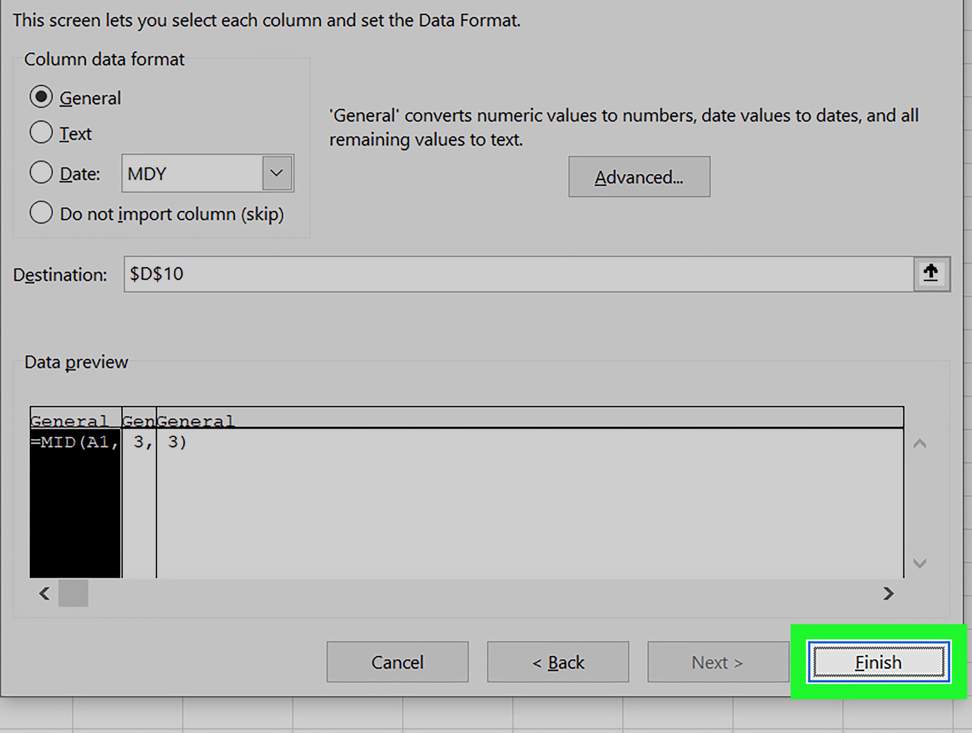
Text to Columns is a classic Excel tool for splitting text into separate columns. It is useful when your text contains consistent delimiters such as commas, tabs, spaces, or hyphens.
To use it, select your data, go to Data > Text to Columns, choose Delimited, select the delimiter, and finish the wizard. If your original value is Blue Shirt - Medium - Cotton, you can split it into separate fields such as product, size, and material. Then you can keep the column you need and remove the rest.
This method is best for quick cleanup when you are comfortable replacing or splitting data. Before using it, copy your original column. Excel is powerful, but it does not always ask, “Are you emotionally attached to this column?” before changing it.
Use Power Query for Repeatable Truncation
Power Query is the best option when you need a repeatable cleanup process. It lets you import data, transform it, and refresh the result later. You can split columns by delimiter, keep characters from the beginning or end, extract text before or after a delimiter, remove unwanted characters, and apply the same steps every time new data arrives.
To start, select your data and go to Data > From Table/Range. In the Power Query Editor, choose your text column, then use options such as Split Column, Extract, or Transform. When finished, load the cleaned data back into Excel.
Power Query may feel heavier than a formula for a small list, but it shines when you process recurring exports, monthly reports, CRM downloads, product catalogs, or any file that keeps arriving in the same messy format. Build the cleanup once, refresh it later, and enjoy the rare spreadsheet luxury of not repeating yourself.
Choosing the Best Excel Text Truncation Method
The best method depends on your data pattern. Use LEFT, RIGHT, and MID when you know exactly how many characters to keep. Use TEXTBEFORE, TEXTAFTER, or LEFT with SEARCH when your text has a reliable delimiter. Use Flash Fill for quick pattern-based work, Text to Columns for fast splitting, and Power Query for repeatable cleanup.
Here is a simple way to decide:
- Need the first 10 characters? Use
LEFT. - Need the last 4 characters? Use
RIGHT. - Need characters from the middle? Use
MID. - Need text before a comma, dash, or slash? Use
TEXTBEFOREorLEFTwithSEARCH. - Need a quick one-time cleanup? Try Flash Fill or Text to Columns.
- Need to repeat the cleanup every week? Use Power Query.
Common Mistakes When Truncating Text in Excel
Mistake 1: Confusing Display Changes with Data Changes
Changing column width or wrapping text does not truncate the actual cell value. It only changes what you see. If another formula references that cell, it still reads the full text. If you truly need shorter data, use a formula or transformation tool.
Mistake 2: Forgetting to Copy and Paste Values
When you use formulas, the output depends on the original data. If you want to replace the original text with the shortened version, copy the formula results and use Paste Special > Values. This preserves the final text without keeping the formulas attached.
Mistake 3: Ignoring Inconsistent Data
Not every row behaves politely. Some rows may be missing a delimiter. Others may have extra spaces or a different code format. Before applying truncation to thousands of rows, test your formula on a sample and scan for errors such as #VALUE!.
Mistake 4: Not Keeping a Backup Column
Always keep the original text somewhere, especially when cleaning imported data. A backup column is cheap insurance. It lets you compare results, fix mistakes, and avoid explaining to your manager that the customer notes disappeared because “Excel seemed confident.”
Practical Examples of Truncating Text in Excel
Example 1: Shorten Product Names for Labels
Suppose your product names are too long for shelf labels. If A2 contains Organic Cotton Crewneck T-Shirt - Navy Blue, you can keep the first 25 characters with:
If you want to avoid cutting a word awkwardly, delimiter-based cleanup may be better. If the size or color always appears after a dash, use:
Example 2: Extract Usernames from Email Addresses
If A2 contains [email protected], use:
The result is:
For older Excel versions, use:
Example 3: Keep File Extensions
If A2 contains quarterly_report.xlsx, you can get the last four characters with:
The result is:
If file extensions vary in length, delimiter logic based on the period may be more accurate.
Experience-Based Tips for Working with Truncated Text in Excel
After working with Excel text cleanup in real-world spreadsheets, one lesson becomes clear: truncation is rarely just about making text shorter. It is usually about making data more useful. A long customer note, product description, or imported code may look harmless, but once you need to filter it, match it, print it, upload it, or turn it into a report, the extra text can become a tiny administrative monster.
The first practical tip is to inspect your data before choosing a method. Do not immediately reach for LEFT(A2,10) just because it works on the first row. Scroll through the column. Look for blanks, longer entries, missing dashes, double spaces, unexpected commas, and values that contain the delimiter more than once. Excel formulas are obedient, not psychic. If the pattern changes, the result changes too.
Second, create a helper column instead of editing the original data directly. Put your truncation formula in a new column, review the output, and only then decide whether to paste the results as values. This habit prevents many small disasters. It also makes troubleshooting easier because you can compare the original text and the shortened text side by side.
Third, name your new columns clearly. A column called Short Name, Product Code, Region Extracted, or Email Username is easier to understand than a mysterious column called Column B. Future you will appreciate the courtesy. Future you has enough problems already.
Fourth, be careful when truncating data that may need to remain unique. For example, shortening customer IDs, invoice numbers, or product SKUs can accidentally create duplicates. Two different values may share the same first eight characters. Before using truncated text as a lookup key, run a duplicate check. A shortened code is useful only if it still identifies the right record.
Fifth, use formulas for live worksheets and Power Query for repeatable imports. If your source values will change and you want the shortened output to update automatically, formulas are convenient. If you receive the same kind of file every week or month, Power Query is usually cleaner. It records the steps and lets you refresh the transformation instead of rebuilding your cleanup process by hand.
Sixth, remember that truncation can remove context. A product name shortened to 20 characters may look tidy, but it might cut off the most important part, such as size, color, or version. Before setting a character limit, test how the output will be used. A dashboard label may need only a short name, while an inventory upload may require the exact model detail.
Seventh, document your logic. You do not need a novel, but a short note such as “Extracts text before first dash” can save confusion later. This is especially helpful in shared workbooks. A spreadsheet without notes can become a puzzle, and not the fun kind with coffee and a rainy window. More like the kind where someone asks why sales data is missing three characters.
Finally, test with edge cases. Try rows with no delimiter, extra delimiter, very short text, blank cells, and unexpected symbols. If your formula breaks, improve it before applying it across the whole dataset. Truncating text in Excel is easy; truncating it safely is the professional move.
Conclusion
Learning how to truncate text in Excel gives you more control over messy data, long labels, imported codes, and worksheet clutter. For predictable text, LEFT, RIGHT, MID, and LEN are reliable workhorses. For text separated by commas, dashes, spaces, or other delimiters, TEXTBEFORE, TEXTAFTER, and SEARCH-based formulas offer smarter extraction. For quick cleanup or repeatable workflows, Flash Fill, Text to Columns, and Power Query can save time without requiring formula gymnastics.
The best approach is the one that matches your data. Count characters when the structure is fixed. Use delimiters when the useful text is separated by a clear marker. Use Excel tools when you need speed, simplicity, or repeatable transformation. Once you understand these three ways to truncate text in Excel, you can clean spreadsheets faster, build better reports, and stop long text from bossing your workbook around.